Real World Example: Expansionary Monetary Policy

US Central Bank, the Federal Reserve (Fed)

IB Economics syllabus: Macroeconomics (expansionary monetary policy)

Using one or more real world examples is essential in your IB Economics Paper 1 exams, part b), 15 mark question to score top marks. If you get a question related to expansionary monetary policy (for example in fighting unemployment or to boost economic growth) you can use the following:

Short version:

During the Financial Crisis, the central bank of the US (the Fed) decreased interest rates (the discount rate) from above 5% to almost 0% (0.25%). As this had still not brought down unemployment enough, while there was a fear of a deflationary development, in Sep 2012 they introduced quantitative easing, pumping $40 billion per month into the economy through buying mortgage-backed securities.

Over the year this has brought down unemployment below 6% by 2016, at which point the Fed decided to start increasing interest rates and scaling down its quantitative easing.

Detailed version – if you really want  to understand:

Lowering the discount rate

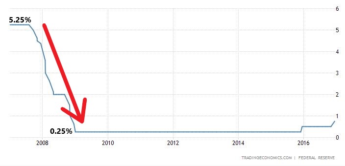
During the Great Financial Crisis, the Fed decreased the discount rate from 5.25% to 0.25% in order to stop the recession and the growing unemployment. This happened between mid-2007 till late 2008. Then they kept the discount rate at place (at 0.25%) for 7 years to make sure firms and households get access to low cost loans.

Figure 1: Discount Rate in the US During and Following the Financial Crisis (2007-2017)

Quantitative easing (QE3)

In Sep 2012, Ben Bernanke, the chairman of the Fed back then announced that the central bank of the US started a quantitative easing cycle. To be more exact, this was the first ever “open-ended” QE programme, meaning that there was no set date for ending it. Instead, the Fed stated that they will continue pouring $40 billion per month into the economy up until unemployment falls to acceptable levels. At the time while unemployment was down from its peak of about 10%, for most of 2012 it remained steadily above 8%, which was not acceptable to the central bank of the US. 3 months after the announcement, they increased the monthly QE to $85 billion. See the results in the below graph about US unemployment.

Figure 2: Unemployment rate in the US During and Following the Financial Crisis (2007-2017)

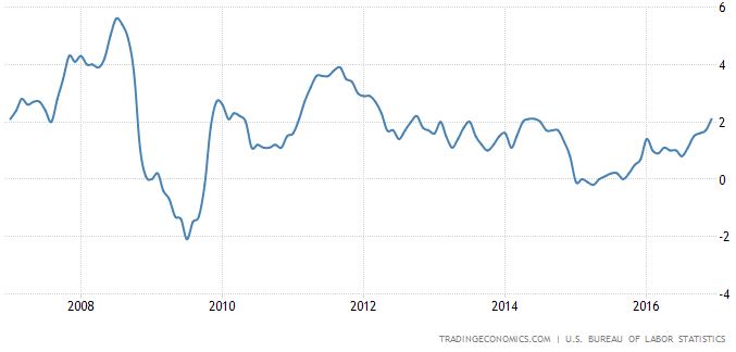
As shown above, cutting the interest rates was not enough, so the Fed took action by implementing quantitative easing. In the following years, unemployment kept decreasing in a steady manner to below 6%. Interestingly, the Fed was not too concerned with inflationary risks as at the time the main goal was to cut unemployment and avoid deflation. Indeed, inflation (see below) has stayed at or below 2% until the end of 2016, while unemployment went below 5% in early 2015 to continue decreasing in the following years. This proves the Keynesian concept that increases in aggregate demand (AD) do not have to be inflationary (shown by a shift of AD to the right on the horizontal section of the Keynesian AS curve).

Figure 3: Inflation in the US between 2007 and 2017

Source of image: Unsplash.com and tradingeconomics for the diagrams

 November 2023 Exam Revision Course

Do you need a little boost with IB Economics?